Oral Bolus Model
For convenience and compliance related reasons, the vast majority of drugs are usually administered via the oral or the extra-vascular route of administration in varying dosage forms.
Consequent to the administration of an oral dosage form to gastric lumen, the drug gets absorbed and enters the systemic circulation from which it will be eliminated. These processes may be diagrammatically presented as follows:
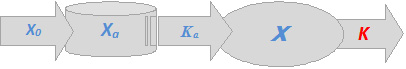
Figure 3. Schematic presentations for plasma conc.-time profiles for a one-compartment intravenous model as per Equation (1.2) (left plot) and (1.3) (right plot), where \(K_a\) is a first order apparent absorption rate constant and \(X_a\) is the quantity of the administered dose that is actually available for absorption. Other parameters have been defined earlier.
Appreciation for the mode of administration of the oral dosage form is critical for the adequate interpretation of this model. If a drug has been administered as bolus manner (i.e. immediate release solid or liquid forms), the absorption rate will be of a first order nature. However, for sustained release form, this rate will be seriously confounded by the release pattern of the drug from the dosage form. In other words, the mode of release of the drug from the dosage form will represent the rate-limiting step in the entire absorption process. This will result in a situation that mimics the intravenous infusion model since both will have the zero input rates in the system.
Based on the above consideration, the mathematical treatment of the orally administered drugs must take into account the nature of the input rate of such drugs from their dosage form. Consequently, two distinct scenarios may be contemplated, as described hereunder.
Oral PK with first-order absorption
Considering the conceptual model as outlined above, a differential expression incorporating the absorption of the gastric and intestinal lumen may be provided as: $$\frac{dX}{dt}=K_a X_a - KX$$ Taking the integral form of this equation will yield the following expression $$X=\frac{K_a FX_0}{K_a-K}(e^{-Kt}-e^{-K_a t})$$ It is noteworthy that the first order elimination does not represent a true description of the absorption process since it does not account for the fraction of that dose that has been subject to this process. This is related to the realization that parts of the administered dose may never be absorbed into the systemic circulation due to the physic-chemical nature of the drug entity. Also, other parts may be lost through various metabolic processes prior to the entry of the drug to the blood stream. For these reasons, any measurements of the absorption rate are an apparent by their very nature.
The above differential equation may be represented in an integral form to estimate the drug concentration in the plasma as a function of time $$C_p=\frac{K_a F X_0}{V_d (K_a - K)}(e^{-Kt}-e^{-K_a t})\label{ref10}\tag{10}$$ The above mathematical model is only valid where the absorption rates are different from the elimination rates, i.e. \(K_a \ne K\).
This model could be used to simulate the plasma conc.-time profile under different conditions. It also represents a unique instance through which the convolution nature of the compartmental PK models could be clearly demonstrated. The concept of convolution is intimately related to most domains of the PK science. This holds true since the magnitude of drug levels in the body are determined by the number of the driving forces consisting any particular PK system. Consequently, it must be realized that the impact of such forces is decided by the magnitude of the exponential terms representing them. With the exception of the one-compartment intravenous model, the evaluation of drug’s plasma conc.-time data implies the deconvolution of convoluted PK systems.
Considering the one-compartment oral model, the magnitude of the time-dependent variable (plasma levels) in this model is determined by a constant value, \(K_a FX_0 /V_d (K_a - K)\), and two driving forces associated with the absorption and elimination processes. The make-up of these two forces consists of the rate constants (\(K_a\) and \(K\)) and a time variable. It is important to emphasize that since these two forces act simultaneously, the interplay of them will ultimately determine the time dependent variable \(C_p\). This signifies that they will continue to have a significant impact on the magnitude of plasma levels in as far as they assume a significant value. Hence, the value of the exponents representing them (i.e. \(e^{-Kt}\) and \(e^{-K_a t}\)) will ultimately determine the magnitude of the plasma level. Since these two exponents consist of a variable time element and two rate constants, it follows that the relative magnitude of either of them, versus the other, will decide whether it is to have the lasting effect in the PK model. This argument provides grounds for various scenarios for the interpretation of the model.
As mentioned earlier the model consists of the absorption and elimination exponents. The magnitude of each component is determined by the time element and their respective rate constants. The rest of the model is a composite constant value incorporating the administered dose and all other PK for any specific drug. In the case of short absorption half-life, the absorption rate constant will be very high which causes a relatively fast absorption of drugs. More pertinent to this is the fact the influence of the absorption exponent will become insignificant thus leaving the elimination exponent to drive the system.
A scenario that represents the most common PK instances for the one-compartment oral model is based on the assumption that the absorption rate constant \(K_a\) is relatively higher than that of the elimination rate constant \(K\). This assumption signifies that the exponential term associated with the absorption process in the above model will approximate zero while the exponent representing the elimination process(s) will continue to assume an infinitesimal value. Thus the model could be reduced to the following equality: $$C_p=\frac{K_a F X_0}{V_d (K_a - K)}e^{-Kt}\text{ for }K_a \ne K \text{ and }K_a \gg K$$ This model implies that the decline in the slope of the plasma conc.-time profile will be indicative of the elimination characteristic of the drug in question. Furthermore, setting the time element within the exponential term in the model to zero will produced a zero-time intercept equivalent to $$C_{p(0)}=\frac{K_a F X_0}{V_d (K_a - K)}\text{ for }K_a \ne K \text{ and }K_a \gg K$$ This intercept is a common term for both the absorption as well as the elimination exponent in the model. For drug with relative short biological half-lives with poor absorption characteristics from the gastro-intestinal tract (GIT), the likelihood exists for foster absorption than elimination rate. This implies that \(K_a \ll K\). In this case the exponent associated with the elimination processes will approximate zero while that representing the absorption process will continue to assume an infinitesimal value. This means that the slope of the terminal segment of the plasma conc.-time profile will be indicative of the absorption properties of the drug. This PK instance is referred as flip-flop kinetics. In this case, the generalized one-compartment oral PK model will reduce, to the following model when the time element becomes significantly large, $$C_p=\frac{K_a F X_0}{V_d (K_a - K)}e^{-K_a t}\text{ for }K_a \ne K \text{ and }K_a \ll K$$
Deconvolution of the Oral Model
As mentioned earlier, one of the fundamental characteristics of many of the PK models is that they are convoluted systems. This is particularly the case with models consisting of more than one exponential term or function. Convolution signifies that although an observed plasma conc.-time data looks like a single profile, such profile represent the outcome of more than one force (or process) determining its ultimate picture. The deconvolution of these systems represent one of the prime concern of the PK science.
Noteworthy, the absorption phase comes to an end when there is no more drug available at the absorption site. This phase far exceeds the observed maximum plasma level which represents a point of time where the elimination and absorption rates are more or less identical. This realization is often overlooked in the PK literature. Irrespective of whether \(K \gg K_a\) or \(K \ll K_a\) one can proceed to assess the drug’s elimination as well as the absorption characteristic. This can be done though the deconvolution procedures which consist of splitting apart the two driving forces comprising the system. This process is called the “Method of Residual” in the PK literature. Other synonyms are also use such as “Curve Stripping” or “Curve Feathering”. The mathematical basis for this process may be outlined as follows:
For simplicity, we may assume that the zero-time intercept \(K_a FX_0/V_d(K_a-K)\). It follows that Equation (\ref{ref1.2}) may be re-written as: $$C_p=Ae^{-Kt}-Ae^{-K_a t}$$ Under usual circumstance, the absorption term will approximate zero which will make the terminal segment of the plasma conc.-time represent the elimination processes. This segment is then extrapolated back to time zero. However, it must be noted that the ascending part of the plasma conc.-time profile represents both the absorption and the elimination processes. Accordingly, if we subtract such quantities from those pertaining to the extrapolated elimination values, the residuals will represent the drug’s absorption characteristics. This is mathematically expressed as follows:
If the plasma levels are subtracted as mention above we get the following equalities: $$C_{p(K)}=Ae^{-Kt}$$ $$-C_{p(K+K_a)}=-Ae^{-Kt}+Ae^{-K_a t}\text{, i.e. }C_{p(K_a)}=Ae^{-K_a t}$$ This implies that the slope of the residual exponent represents the absorption properties if, and only if, the elimination rate is relatively faster than the absorption rate. This holds true the other way round when a flip-flop situation exists. A typical presentation for a flip-flop situation is shown hereunder.
Estimation of \(T_{max}\) and \(C_{max}\)
For drug whose onset of action assumes distinct therapeutic significance, it is always desirable to determine the length of time within with the drug entity elicits its therapeutic response of efficacy. This is true for a wide variety of drugs like nitro glycerides and analgesics. On the other hand, it is often needed to assess the maximum drug levels attained in the body especially if such levels are associated with adverse drug effects. Estimation of such levels provides an important measure for the design and consequent adjustment of dosing regimen.
In order that the maximum plasma level is estimated, one needs to determine the time at which such plasma level is attained. This point of time occurs when no further increase in the drug level occurs, rather it start to decline. In other words, the slope of the ascending part of the plasma profile tends to level, or approximates a zero value. This situation could be mathematically expressed by differentiating the concentration term in Equation (\ref{ref10}) with respect to time and setting the resultant term equal to zero the time element set \(t_{max}\). This is demonstrated as follows:
The natural logarithm for both side of the latter expression may be taken and further solved for \(T_{max}\) as shown hereunder: $$T_{max}=\frac{1}{K_a-K} \ln \frac{K_a}{K}$$ Once \(T_{max}\) has been estimated, it could be substituted in Equation (\ref{ref10}) so that an estimate for \(C_{max}\) is obtained.
PK of Oral Multiple Dosing
A mathematical model for oral multiple dosing could be formulated according to Dost’s relevant generalization. This is done by multiplying each exponential term in the model for a single oral bolus mode of administration as given in Equation \ref{3.1}). Hence, $$C_N=\frac{K_a F X_0}{V_d (K_a - K)}\left( \frac{1-e^{-NK\tau}}{1-e^{-K\tau}}e^{-Kt} - \frac{1-e^{-NK_a\tau}}{1-e^{-K_a\tau}}e^{-K_at} \right)$$ This is a full-fledge model can be used to determine the drugs plasma level after any number \(N\) of doses as well as at any time point during the dosing interval \(\tau\). It could be also rewritten to estimate specific instances such as the maximum and minimum plasma levels after any dose or once steady state has been attained according to the following equations: $$C_{max}^{ss}=\frac{K_a F X_0}{V_d (K_a - K)}\left( \frac{e^{-Kt_{max}^{ss}}}{1-e^{-K\tau}} - \frac{e^{-K_a t_{max}^{ss}}}{1-e^{-K_a\tau}} \right)$$ $$C_{min}^{ss}=\frac{K_a F X_0}{V_d (K_a - K)}\left( \frac{e^{-K\tau}}{1-e^{-K\tau}} - \frac{e^{-K_a \tau}}{1-e^{-K_a\tau}} \right)$$ In addition to the above mentioned plasma levels estimates, the average plasma concentration after the administration of any dose, or at steady state could be also estimated. In this regard, one has to resort to a globally accepted definition of this parameter which is given as the product of the area under the plasma conc.-time curve divided by the dosing interval. It has been earlier verified that for a one-compartment intravenous bolus model the \(AUC_{0-\tau}^{ss}\)is operationally equivalent to the \(AUC_{0-\infty}^{N=1}\). This concept has been applied to the one-compartment oral model. However, examination of the areas estimates according to the equations provided below would invalidate such generalization. $$AUC_{0-\tau}^{ss}=\frac{FX_0K_a\left[ (1-e^{-K\tau}) + K (e^{-K_a\tau}-1)\right]}{KV_d(K_a-K)(1-e^{-K\tau})}\text{ and }AUC_{0-\infty}^{N=1}=\frac{FX_0}{KV_d}$$
Time to attain maximum plasma level \(T_{max}\) where \(K_a \ne K\)
$$T_{max}^N=\frac{1}{K_a-K}\ln \left[ \frac{K_a}{K} \frac{1-e^{-K\tau}}{1-e^{-nK\tau}} / \frac{1-e^{-K_a\tau}}{1-e^{-nK_a\tau}} \right]$$ $$T_{max}^{ss}=\frac{1}{K_a-K}\ln \left[ \frac{K_a}{K} \frac{1-e^{-K\tau}}{1-e^{-K_a\tau}} \right]=t_p^{ss}\text{ ... for }K_a \ne K$$ Once the time required to attain a maximum plasma level at steady state has been determined, the maximum plasma level could be estimated as: $$C_{max}^{ss}=\frac{K_a F X_0}{V_d (K_a - K)}\left( \frac{e^{-Kt_{p(ss)}}}{1-e^{-K\tau}} - \frac{e^{-K_a t_{p(ss)}}}{1-e^{-K_a\tau}} \right)$$ $$C_{min}^{ss}=\frac{K_a F X_0}{V_d (K_a - K)}\left( \frac{e^{-K\tau}}{1-e^{-K\tau}} - \frac{e^{-K_a \tau}}{1-e^{-K_a\tau}} \right)$$ $$C_{max}^{ss}-C_{min}^{ss}=\frac{K_a F X_0}{V_d (K_a - K)} \left( \frac{e^{-Kt_p^{ss}}-e^{-K\tau}}{1-e^{-K\tau}}- \frac{e^{-K_at_p^{ss}}-e^{-K_a\tau}}{1-e^{-K_a\tau}}\right)$$ Considering that the entity \(t_p^{ss}\) has been defined above for any dosing interval, a new dosing interval that will produce a newly defined maximum and minimum plasma levels could be estimate by numerical iteration techniques. $$C_{max}^{ss}=\frac{K_a F X_0}{V_d (K_a - K)} \left( \frac{e^{-KT_{max}^{ss}}}{1-e^{-K\tau}}- \frac{e^{-K_aT_{max}^{ss}}}{1-e^{-K_a\tau}} \right)$$ $$C_{min}^{ss}=\frac{K_a F X_0}{V_d (K_a - K)} \left( \frac{e^{-k\tau}}{1-e^{-K\tau}}- \frac{e^{-K_a\tau}}{1-e^{-K_a\tau}} \right)$$
Magnitude of Fluctuation
As defined earlier, the degree of fluctuation may be obtained by dividing the maximum by the minimum plasma levels at steady state. Since these have been defined above, the degree of fluctuation may be given as: $$\frac{C_{max}^{ss}}{C_{min}^{ss}}=\frac{\frac{K_a F X_0}{V_d (K_a - K)} \left( \frac{e^{-KT_{max}^{ss}}}{1-e^{-K\tau}}- \frac{e^{-K_aT_{max}^{ss}}}{1-e^{-K_a\tau}} \right)}{\frac{K_a F X_0}{V_d (K_a - K)} \left( \frac{e^{-K\tau}}{1-e^{-K\tau}}- \frac{e^{-K_a\tau}}{1-e^{-K_a\tau}} \right)}$$ This equation may be simplified as follow: $$MoF=\frac{\frac{e^{-KT_{max}^{ss}}}{1-e^{-K\tau}}- \frac{e^{-K_aT_{max}^{ss}}}{1-e^{-K_a\tau}}}{\frac{e^{-K\tau}}{1-e^{-K\tau}}- \frac{e^{-K_a\tau}}{1-e^{-K_a\tau}}}$$ $$MoF=\frac{e^{-KT_{max}^{ss}}(1-e^{-K_a\tau}) - e^{-K_aT_{max}^{ss}}(1-e^{-K\tau})}{e^{-K\tau}(1-e^{-K_a\tau}) - e^{-K_a\tau}(1-e^{-K\tau})}$$ $$MoF=\frac{e^{-KT_{max}^{ss}}-e^{-K_aT_{max}^{ss}}+e^{-K_aT_{max}^{ss}}e^{-K\tau}}{e^{-K\tau}+e^{-K_a\tau}e^{-K\tau}}$$ If the dosing interval is set so that consecutive dosing are administered in the post absorptive phase, the above expression may approximated by the following relationship: $$MoF=\frac{e^{-KT_{max}^{ss}}-e^{-K_aT_{max}^{ss}}(1-e^{-K\tau})}{e^{-K\tau}}$$ $$e^{-K\tau}=\frac{e^{-KT_{max}^{ss}}-e^{-K_aT_{max}^{ss}}}{MoF-e^{-K_aT_{max}^{ss}}}$$ $$\tau_{new}=\frac{1}{K}\ln \frac{MoF-e^{-K_aT_{max}^{ss}}}{e^{-KT_{max}^{ss}}-e^{-K_aT_{max}^{ss}}}$$ This is due to the fact that all exponential terms associated with the expression \(e^{-K_a\tau}\)will become insignificant; hence they will cancel from the previous equations.
Average Plasma Concentration \(K_a \ne K\)
Estimation of the average plasma levels requires that the area under the plasma conc.-time curve \(AUC\) be determined. This could be done for any dose under during a dosing regimen. After a single dose, \(AUC\) from time zero to infinity may be obtained by integration the plasma levels as provided hereunder: $$\int_0^\infty C_p\,dt=\frac{K_aFX_0}{V(K_a-K)}\left(\frac{1}{K}-frac{1}{K_a}\right)=\frac{FX_0}{VK}$$ This equation clearly signifies that the \(AUC\), or the so called total exposure of the body to the administered drug, is a function of its elimination characteristics. Assuming complete bioavailability (i.e. \(F\) equals unity), the above expression becomes identical to that obtained after intravenous bolus administration. Also, the area under the plasma conc.-time curve during any dosing interval under multiple dosing conditions may be estimated by integration the equation representing the relevant multiple dosing model as follows: $$\int_0^\tau C_p^N\,dt=\frac{K_aFX_0}{V_d(K_a-K)}\left[ \left(\frac{1-e^{NK_a\tau}}{1-e^{K_a\tau}}\right)\frac{e^{-K_a\tau}}{K_a} - \left(\frac{1-e^{NK\tau}}{1-e^{K\tau}}\right)\frac{e^{-K\tau}}{K} + \left(\frac{1-e^{NK\tau}}{1-e^{K\tau}}\right)\frac{1}{K} - \left(\frac{1-e^{NK_a\tau}}{1-e^{K_a\tau}}\right)\frac{1}{K_a} \right]$$ Simplification of the above equation produces the expression: $$\int_0^\tau C_p^N\,dt=\frac{FX_0}{KV_d}\left( 1+ \frac{Ke^{-NK_a\tau}}{K_a-K}-\frac{K_ae^{-NK\tau}}{K_a-K} \right)$$ It is evident that the above expression could be further simplifies as the administered number of doses \(N\) becomes larger, or at steady state. In this case the bracketed terms associated with the exponents become very insignificant and the above equation reduces to the following: $$\int_0^\infty C_p^N\,dt=\frac{FX_0}{KV_d}$$ The preceding mathematical consideration clearly demonstrate that the area under the plasma conc.-time curve, from tine zero to infinity, obtained after the administration of a single dose is identical to the area under the plasma conc.-time curve during any dosing interval at steady state.
Defining the Degree of Fluctuation (Swing)
In the of an oral bolus model, the degree of fluctuation as measured by the swing, we have the three PK metrics defining the swing. These are the maximum, minimum and average plasma levels at steady state. Their respective values are provided below: $$C_{max}^{ss}=\frac{K_a F X_0}{V_d (K_a - K)}\left( \frac{e^{-Kt_{p(ss)}}}{1-e^{-K\tau}} - \frac{e^{-K_a t_{p(ss)}}}{1-e^{-K_a\tau}} \right)$$ Hence, the degree of fluctuation may be given as: $$C_{min}^{ss}=\frac{K_a F X_0}{V_d (K_a - K)}\left( \frac{e^{-K\tau}}{1-e^{-K\tau}} - \frac{e^{-K_a \tau}}{1-e^{-K_a\tau}} \right)\text{ and }C_{av}^{ss}=\frac{FX_0}{\tau KV_d}$$ This readily rearranges after cancellation of common terms to the following expression: $$DoF_{swing}=\frac{\tau KK_a}{K_a-K}\left[ \left( \frac{e^{-Kt_p^{ss}}}{1-e^{-K\tau}} - \frac{e^{-K_a t_p^{ss}}}{1-e^{-K_a\tau}} \right) - \left( \frac{e^{-K\tau}}{1-e^{-K\tau}} - \frac{e^{-K_a \tau}}{1-e^{-K_a\tau}} \right) \right]$$ $$DoF_{swing}=\frac{\tau KK_a}{K_a-K}\left( \frac{e^{-Kt_p^{ss}}-e^{-K\tau}}{1-e^{-K\tau}}+\frac{e^{-K_a\tau}-e^{-K_at_p^{ss}}}{1-e^{-K_a\tau}} \right)$$ Irrespective of the relative magnitude of \(K\) or \(K_a\), if the dosing interval is set at more than six hours, the above expression will approximate the following: $$DoF_{swing}=\frac{\tau KK_a}{K_a-K}(e^{-Kt_p^{ss}}-e^{-K_at_p^{ss}})$$
Targeting Therapeutic Ranges
For drugs administered by the oral route a dosing regimen (a dose and dosing interval) may be theoretically determined so that a pre-defined plasma range is attained. Although the mathematical basis for determining such regimens does no differ from that adopted for other routes, the presence of an absorption phase makes it a little different. This is related to the confounding effect of the absorption rate constant to the PK definition of the targeted therapeutic range. Differences in such rate will influence the time required to attain a maximum plasma level which will further affect the estimation of the magnitude of such level. The consequent estimation if the desired therapeutic plasma range will be also affected.
This is further complicated by the realization that the time required to attain a maximum plasma level after a single dose will differ from the same at steady state. \(T_{max}^{N=1}\) after the first dose is given as: $$T_{max}^{N=1}=\frac{1}{K_a-K}\ln\frac{K_a}{K}$$ At steady state conditions \(T_{max}^{ss}\) may be given as follows: $$T_{max}^{ss}=\frac{1}{K_a-K}\ln\frac{K_a(1-e^{-K\tau})}{K(1-e^{-K_a\tau})}$$ It has been demonstrated that \(C_{max}\) after the first dose may be estimated according to the following equation: $$C_{max}^{(N=1)}=\frac{FX_0}{V}e^{-KT_{max}}$$ Similarly, the maximum as well as the minimum plasma levels at steady state may be expressed as: $$C_{max}^{ss}=\frac{FX_0}{V}\left( \frac{e^{-KT_{max}}}{1-e^{-K\tau}} \right)\text{, }C_{min}^{ss}=\frac{FX_0}{V}\left( \frac{e^{-K\tau}}{1-e^{-K\tau}} \right)$$ The range of peak to trough fluctuation could be accordingly estimated as: $$\frac{C_{max}^{ss}}{C_{min}^{ss}}=\frac{e^{-KT_{max}^{ss}}}{e^{-K\tau}}$$ The dosing interval associated with such range is then readily determined as a function of this range: $$e^{-KT_r}=\frac{C_{min}^{ss}e^{-KT_{max}^{ss}}}{C_{max}^{ss}}\text{, }\tau=\frac{1}{K}\ln \frac{C_{max}^{ss}}{C_{min}^{ss}e^{-KT_{max}^{ss}}}$$ For a newly desired range a new dosing interval could be estimated as: $$\tau_{new}=\frac{1}{K}\ln \frac{C_{maxT}^{ss}}{C_{minT}^{ss}e^{-KT_{max}^{ss}}}$$ Other less precise expression has been reported in the PK literature $$\tau_{new}=\frac{1}{K}\left( \ln C_{max} - \ln C_{min} \right) + T_{max}\text{ or }\tau_{new}=\frac{1}{K}\ln \frac{MoF-e^{-K_aT_{max}^{ss}}}{e^{-KT_{max}^{ss}}-e^{-K_aT_{max}^{ss}}}$$ The approximate dose needed to bring the plasma levels for the desired SS therapeutic window may be roughly estimated according to the newly defined dosing interval as provided above: $$X_0=\frac{C_{min}^{ss}V_d(K_a-K)}{K_aF}\left( \frac{e^{-K\tau_{new}}}{1-e^{-K\tau_{new}}} - \frac{e^{-K_a\tau_{new}}}{1-e^{-K_a\tau_{new}}} \right)$$