Intravenous Bolus Model (IVB)
For drugs that confer upon the body the characteristic of a one-compartment model, and are administered by an intravenous bolus fashion, a conceptual model could be outlined to describe the administration, and the consequent elimination, of the drug from the body:
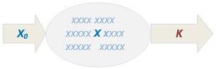
Figure 1. A schematic presentation for a one-compartment intravenous model.
According to this model, the drug is subcutaneously, intramuscularly or intravenously administered as one shot into the systemic circulation. It will be then rapidly distributed to different parts of the body in a very short period of time. Usually, this happens within few minutes after the administration of the dose. This fast distribution of the drug is associated with simultaneous clearance via different renal and hepatic elimination processes. There is ample evidence that such processes occur at a first order rate which is designated by an overall rate constant that represents the totality of the elimination processes for any drug substance.
The differential mathematical expression depicting the amount of the drug remaining in the body with time could be expressed as: $$\frac{dX}{dt}=-KX\label{ref1.0}\tag{1.0}$$ This equation suggests that only a fraction amount of the drug remaining in the body gets elimination per time unit. Hence, it only depicts the ever-decreasing value of the elimination rate. The integral counterpart of Equation (\ref{ref1.0}) may be expressed as follow: $$X=X_0e^{-Kt}\label{ref1.1}\tag{1.1}$$ Equation (\ref{ref1.1}) may be expressed in concentration terms as: $$C_p=\frac{X_0}{V_d}e^{-Kt}\label{ref1.2}\tag{1.2}$$ where \(C_p\) represents the plasma concentration attained at time \(t\), after the administration of a single dose \(X_0\), \(V\) is volume of distribution and \(K\) is elimination rate constant.
Representation of Equation (\ref{ref1.2}) in the logarithmic (base 10) or in the natural logarithmic form will respectively give Equations (\ref{ref1.3}) and (\ref{ref1.4}) as shown below, $$\log(C_p)=\log\left(\frac{X_0}{V_d}\right)-\frac{Kt}{2.303}\label{ref1.3}\tag{1.3}$$ $$\ln(C_p)=\ln\left(\frac{X_0}{V_d}\right)-Kt\label{ref1.4}\tag{1.4}$$ Equation (\ref{ref1.4}) may be also expressed in natural logarithmic terms as: $$\ln(C_p)=\ln(C_0)-Kt\label{ref1.5}\tag{1.5}$$
All the above Equation (\ref{ref1.5}) demonstrates that the decline of the logarithmically transformed values of plasma levels, with respect to time, occurs in a linear fashion. This implies the representation of such value on a semi-logarithmic scale will produce a straight line with a slope equivalent to the elimination rate constant \(K\) and a zero-time intercept given as: $$\ln(C_{p(0)})=\ln\left(\frac{X_0}{V_d}\right)\label{ref1.6a}\tag{1.6a}$$ $$C_{p(0)}=\frac{X_0}{V_d}\label{ref1.6b}\tag{1.6b}$$
The Volume of Distribution
The distribution characteristics of drugs constitute one of the major concerns in PK science. It represents a measure of the manner by which drugs get distributed in different parts of the body after its administration. It also reflects to what extent drugs get distributed in the extra-vascular space. For poorly distributed drugs, administered doses tend to remain in the system circulation. This is usually interpreted by assuming that such drugs have low volume of distribution. By contrast, drugs having higher volume of distribution tend to disappear from the circulation to various parts of the body. This may be related to the fact that such drugs possess higher affinity to proteins of the extra-vascular space compared to those circulating in the plasma.
A generalized definition to the volume of distribution may be formulated as a proportionality constant that relates the plasma concentration of the drug, at any point in time, to the total amount of the drug in the body at that particular point, i.e. \(V_d=(X_t/C_t)\). According to this definition of the volume of distribution, lower plasma levels of different drugs are indicative of higher magnitude of \(V_d\).
It should be noted that the same dose of drugs I, II and III was administered and the resulting plasma levels were measured at the same time following the drug intake. As shown above, each cylindrical shape represents the volume of distribution for one of the three drugs. The magnitude of this parameter may range from the actual size of the plasma (0.06 - 0.07 liter/kg body weight) to thousands of liters. This implies that, for neonates and infants, a volume term could be estimated at less than unity (i.e. one liter).
Reliable estimates of the volume terms are extremely important, especially within the context of dosage regimen individualization and/or the estimation of the loading dose. Erroneous volume estimates would jeopardize the ability to correctly predict the desired levels of the drug in the body.
The assessment of the distribution properties of drug is best conducted consequent to their administration via the intravenous bolus route. Drug conc.-time profiles obtained though monitoring the drug levels in the plasma are the least affected, or confounded, by other kinetic processes like absorption. The presence of such process will preclude accurate estimation of the distribution process or the volume of distribution. Different approaches have been used for the estimation of the volume terms from the plasma conc.-time data after intravenous bolus (IVB) administration. These consist either of graphic or numerical estimation procedures.
Determination of \(V_d\) Using Estimates of \(AUC\)
This method may be more reliable than the method mentioned in Equation (\ref{ref1.6b}) since it is based on the entire plasma conc.-time profile. Estimates of the area under the plasma conc.-time profile may be determined by integrating the plasma level presented in Equation (\ref{ref1.1}) from time zero to infinity. It could be verified that such integration produces the following equality: $$\int^{\infty}_0 C_p\,dt = \frac{X_0}{KV_d}$$ Rearrangement of this expression, or solving it for Vd gives the following: $$V_d=\frac{X_0}{K\int^{\infty}_0 C_p\,dt} = \frac{X_0}{K(AUC_{0 \to \infty})}\label{ref1.7}\tag{1.7}$$
The area under the plasma conc.-time curve from time zero to infinity \(AUC_{0 \to \infty}\) could be represented by the summation of area of the plasma conc.-time profile from time zero to the last sampling point \(AUC_{0 \to t}\) and the area from the last sampling point to infinity \(AUC_{t \to \infty}\) $$AUC_{0 \to \infty}=AUC_{0 \to t}+AUC_{t \to \infty}$$ The first term in the above equation could be estimated as according to the linear trapezoidal rule expressed as: $$AUC_{0 \to t}=\sum_{i=0}^{n-1}\frac{t_{i+1}-t_i}{2}(c_i+c_{i+1})\label{ref1.8}\tag{1.8}$$ The second term may be computed as: $$AUC_{t \to \infty}=\frac{C_{p(\text{last})}}{K}$$
Once the slope, or the elimination rate constant \(K\) has been determined on the logarithmic scale and the \(AUC_{0 \to \infty}\) has been estimated on the Cartesian (rectilinear) scale, the volume of distribution could be computed as shown in Equation (\ref{ref1.7}).
The Biological Half-life
The biological or elimination half-life \(t_{0.5}\) of drugs is an important PK metric that accounts for the duration of the sojourn of an administered dose of a drug in the body. It is also a parameter that helps in estimating the accumulation of the drugs upon repeated dosing as well as the frequency of such dosing.
The elimination half-life could be defined as the time required for any quantity available in the body, at any time, to be decreased to half its value. Using Equation (\ref{ref1.2}), this can be exemplified by assuming that an initial quantity \(X_0\) equivalent to 50 mg was reduced to half its value (i.e. the quantity remaining in the body became 25 mg). It follows that: $$X=X_0e^{-Kt}$$ $$25=50e^{-Kt_{0.5}}$$ $$0.5=e^{-Kt}\text{ or } \ln0.5=-Kt_{0.5}$$ $$\text{Since }\ln0.5=-\ln2\text{, then }t_{0.5}=\frac{\ln2}{K}$$
The mathematical expression given in the above section (Equations (\ref{ref1.2}), (\ref{ref1.3}) and (\ref{ref1.4})) provide basis for the computation of many useful PK metrics that have distinct clinical signification. Although drug plasma levels represent a general concern within the domain of PK science, the magnitude of drug accumulation, upon repetitive dosing, remains the most important aspect of drug therapy. In as much as accumulation of drugs in the body may be related to their therapeutic efficacy, it is also linked to its adverse effects. A so called Therapeutic Window (TW) has been established for a large number of drug entities. The concept of a TW defines a maximum level beyond which adverse may effects set in, and a minimum level below which the desired therapeutic effect will be lost. Biological half-lives of drugs vary from few minutes (4.0 - 5.0 for insulin), to several hours, days or even weeks.
In addition to the magnitude of drug accumulation consequent to repeated dosing, the degree of fluctuation in drug plasma levels may have an impact on the therapeutic outcome. The relative ratio of peak to trough plasma level represents a direct measure of the degree of fluctuation. This issue constitutes concern for clinicians as well as drug regulatory bodies at an international scale.
Multiple Dosing of IV Bolus Model
For drugs administered on repeated or multiple dosing bases, in the long run a maximum, minimum or average plasma levels will reach stable levels. Time required for such level to be reach is solely determined by the drug's elimination characteristics irrespective of the dosing frequency. As demonstrated above, the magnitude of these levels is a function of these characteristics, as well as the dosing rate (administered doses and the dosing interval). This PK model could be expressed in a generalized manner suited to construct the plasma conc.-time profiles after the administration of a single dose or under multiple dosing conditions. $$C_p^N=\frac{X_0}{V_d}\left(\frac{1-e^{-NK\tau}}{1-e^{-K\tau}}\right)e^{-Kt}\label{ref1.9}\tag{1.9}$$ The model presented in Equation (\ref{ref1.9}) allows the estimation of plasma drugs levels, during any dosing interval, at any \(N\) number of doses. The bracketed quantity represents what could be called a multiple dosing factor (MDF) which determines the magnitude of accumulation of the drug in the body when repetitive doses are administered at regular time intervals. Equation (\ref{ref1.9}) could be readily transformed to an expression suited for a single dose by setting \(N\) (the number of doses) to unity.
Maximum and minimum plasma levels could be estimated during multiple dosing, at any number of doses, by setting the time in the decay exponent to zero (the start of the new dose) or to \(\tau\) (the end of the dosing interval). This will respectively produce Equations (\ref{ref1.9a}) and (\ref{ref1.9b}) as shown below $$C_{p(\text{max})}^N=\frac{X_0}{V_d}\left(\frac{1-e^{-NK\tau}}{1-e^{-K\tau}}\right)\label{ref1.9a}\tag{1.9a}$$ $$C_{p(\text{min})}^N=\frac{X_0}{V_d}\left(\frac{1-e^{-NK\tau}}{1-e^{-K\tau}}\right)e^{-K\tau}\label{ref1.9b}\tag{1.9b}$$ These equations may also be transformed to account for the estimation of drug plasma levels under steady state situations. Under these conditions, the expression \(e^{-NK\tau}\) approximate zero as \(N\) tends to higher values, hence, $$C_p^{ss}=\frac{X_0}{V_d}\left(\frac{1}{1-e^{-K\tau}}\right)e^{-Kt}\label{ref1.9c}\tag{1.9c}$$ The maximum and minimum plasma levels at steady state could be also estimated according to equations (\ref{ref1.9d}) and (\ref{ref1.9e}) respectively, $$C_{p\text{max}}^{ss}=\frac{X_0}{V_d}\left(\frac{1}{1-e^{-K\tau}}\right)\label{ref1.9d}\tag{1.9d}$$ $$C_{p\text{min}}^{ss}=\frac{X_0}{V_d}\left(\frac{1}{1-e^{-K\tau}}\right)e^{-K\tau}\label{ref1.9e}\tag{1.9e}$$ These two equations give measures of the steady state maximum and minimum plasma levels under multiple dosing conditions. While the maximum level is what is obtained immediately after the administration of a new dose, the minimum level is what is measured prior to such administration.
Attainment of Steady State (SS) Plasma Levels
It is obvious from the above multiple dosing equations that it is possible to determine drug levels in the plasma, during the dosing interval, after any number of administered doses as well as under SS condition. For the latter state to be reached the expression \(e^{-NK\tau}=e^{0.693N(\tau/t_{0.5})}\) must become very insignificant or approximates a zero value. This occurs when the number of doses \(N\) becomes sufficiently large. Irrespective of the number of administered doses, or the dosing interval such situation can only occur when the elapsed time, after the initiation of dosing regimen, approximate seven biological half-lives. Also, it is possible to mathematically determine the time required for a fraction of the SS (\(f_{ss}\)) to be reached. This could be done by dividing any plasma level metric attained after a certain number of doses by its corresponding SS metric. This could be mathematically expressed as: $$f_{ss}=\frac{C^N_{\text{max}}}{C^{ss}_{\text{max}}}=\frac{X_0}{V_d}\left(\frac{1}{1-e^{-K\tau}}\right) / \left(\frac{1-e^{-NK\tau}}{1-e^{-K\tau}}\right)$$ Cancellation of common term and simplification gives the following: $$f_{ss}=1-e^{-NK\tau}\text{, or }1-f_{ss}=e^{-NK\tau}$$ In natural logarithmic terms, this expression could be re-written as: $$-NK\tau=\ln(1-f_{ss})\text{, or }-N\tau=1.44 \times t_{0.5}\ln(1-f_{ss})$$ The expression \((-N\tau)\) in the above equation represents the length of time in terms of the number of doses and the dosing interval. It is evident that this parameter is directly proportional to the biological half-life of the drug. This situation is detailed in the following section.
The Loading Dose (\(X_{LD}\))
The therapeutic efficacy for many drugs is generally associated with certain plasma level. Accordingly, therapeutic windows have been determined for such drugs. However, when the biological half-life of a drug is relatively long, it will take a considerable time for the plasma levels to reach their therapeutic window. In general, it will take about four biological half-lives to reach 90% of the drug’s steady state levels in the body.
The estimation of the loading dose should be done in a way to ensure the minimum plasma level it will produce towards the end of the first dosing interval will be identical to the predicted minimum level attained at steady state. This could be mathematically expressed, for intravenous bolus dosing as: $$\frac{X_L}{V_d}e^{-K\tau}=\frac{X_0}{V_d}\left(\frac{e^{-K\tau}}{1-e^{-K\tau}}\right)$$ Cancellation of the common term and re-arrangement of this equation give the following: $$\frac{X_{LD}}{X_0}=\left(\frac{1}{1-e^{-K\tau}}\right)\text{ or }X_{LD}=X_0 \times MDF$$ where \(MDF\) is defined as the multiple dosing factor, or the accumulation ratio (see next section), for a one-compartment model drug administered by an intravenous bolus mode.
Drugs Accumulation Ratio (\(AR\))
A direct measure of the drug accumulation in the body could be estimated as a ratio between the maximum (or minimum) plasma levels attained after the administration of a single dose to their corresponding values at steady state. $$AR=\left(\frac{1}{1-e^{-K\tau}}\right)\frac{X_0}{V_d} / \frac{X_0}{V_d}$$ Cancellation of common terms in the above equation yields the following expression that constitutes a measure of the degree of drug accumulation for a one-compartment model drug administered by an intravenous bolus mode. $$AR=\frac{1}{1-e^{-K\tau}}=1 / 1-e^{-0.693\frac{\tau}{t_{0.5e}}}$$
Average Plasma Concentration, \(C_{p(av)}\)
Although the therapeutic efficacy of certain drugs is often associated with maximum and a minimum plasma levels as mentioned above, the average plasma concentration would represent a superior PK indicator to such efficacy. A definition for this metric is usually related to the area under the plasma conc.-time curve (AUC) divided by the dosing interval. AUC could be determined by integration of Equation (\ref{ref1.2}) from time zero to infinity after the administration of a single dose, hence $$\int^{\infty}_0 C_p\,dt = \frac{X_0}{KV_d}$$ Consequently, the average plasma concentration is estimated as: $$C_p = \frac{X_0}{\tau K V_d}$$ However, under multiple dosing, Equation (\ref{ref1.1}) must be adjusted in order to account for this situation, by multiplying it by Dost’s multiple dosing factor \((1-e^{-NK\tau}/1-e^{-K\tau})\): $$C_p = \frac{X_0}{V_d}\left(\frac{1-e^{-NK\tau}}{1-e^{-K\tau}}\right)e^{-Kt}$$ This above equation may be integrated from time zero to end of the dosing interval. Details of this integration are provided below: $$C_{av}^N=\frac{\int_0^\tau C_p^N}{\tau}=\frac{X_0}{\tau K V_d}(1-e^{-NK\tau})\label{ref1.10}\tag{1.10}$$ Equation (\ref{ref1.10}) indicates that the average plasma levels \(C_{av}^N\), as a function of the area under the plasma conc.-time curve, varies with repetitive dosing. The magnitude of \(C_{av}^N\) is determined by a constant quantity \((X_0 / \tau K V_d)\) for any multiple dosing situation which is multiplied by a variable quantity \((1-e^{-NK\tau})\). This variable quantity reaches its maximum level as the exponential term \( e^{-NK\tau}\) approximates zero as the number of doses \(N\) tends to increase. In this case Equation 1.6 reduces to the following expression: $$C_{av}^{ss}=\frac{\int_0^\tau C_p^{ss}}{\tau}=\frac{X_0}{\tau K V_d}=\frac{C_0}{\tau K}=C_0 \times 1.44\frac{t_{0.5}}{\tau}\label{ref1.13}\tag{1.13}$$ where \(C_{P(0)}\) is defined as the zero-time intercept of the plasma conc.-time profile.
As implied by Equation (\ref{ref1.13}), the value of \(C_{p(av)}^{ss}\) is a constant quantity that could be only attained at what has been conventionally called the steady state situation. The magnitude of such quantity is a function of the drug’s elimination properties as well as the dosing interval. This implies that the average plasma concentration at steady state is proportional to the biological half-life if the drug and inversely proportional with the dosing interval.
Magnitude of Fluctuation (\(MoF\))
There are different measures to assess the fluctuation of drug in the body at steady state. This can be expressed, in simplistic term as the ratio of the maximum to the minimum levels attained under SS condition as shown below, $$MoF = \frac{C_{p(\text{max})}^{ss}}{C_{p(\text{min})}^{ss}}=\frac{X_0}{V_d}\left(\frac{1}{1-e^{-K\tau}}\right) / \frac{X_0}{V_d}\left(\frac{1}{1-e^{-K\tau}}\right)e^{-K\tau}$$ $$MoF = \frac{1}{e^{-K\tau}}=e^{K\tau}\text{, or }\ln MoF=\frac{\tau}{t_{0.5}}ln2\label{ref1.14}\tag{1.14}$$ Equation (\ref{ref1.14}) indicates that the degree of fluctuation could be minimized by decreasing the length of the dosing interval.
The Degree of Fluctuation (\(DoF_{swing}\))
Official measures have been suggested for the assessment of the degree of fluctuation. One such measure is called the swing, which relates the difference between the maximum and minimum plasma levels to the average plasma concentration at steady state in the following fashion: $$DoS_{swing} = \frac{X_0}{V_d}\left(\frac{1}{1-e^{-K\tau}}\right) - \frac{X_0}{V_d}\left(\frac{e^{-K\tau}}{1-e^{-K\tau}}\right) / \frac{X_0}{\tau K V_d}$$ Cancellation of the common and rearrangement of the above expression produces the following relationship: $$DoS_{swing} = \left(\frac{1}{1-e^{-K\tau}}\right) - \left(\frac{e^{-K\tau}}{1-e^{-K\tau}}\right) / \frac{1}{\tau K}=\frac{\tau K}{1-e^{-K \tau}}(1-e^{-K \tau})=\tau K=0.693\frac{\tau}{t_{0.5}}$$ This relationship suggests that the degree of fluctuation is a function of the elimination characteristics and the dosing frequency.
Targeting Therapeutic Ranges
Conventionally, clinical practitioners aim at multiple dosing regimens that would guarantee a maximum plasma level is not exceeded or that plasma levels are maintained above a minimum clinically concentration.
For drugs that have a well-established therapeutic window, it is often desirable to will produce plasma drug levels that falls within such window. This implies that such levels must not exceed a maximum, or decline to less than a minimum, predefined level. Since we generally have a prior knowledge of the therapeutic window of certain drugs, the relationship between the boundaries of this window could be determined according to the elimination characteristic as well as the dosing frequency.
A new dosing interval may be defined on the basis of the desired levels of \(C_{\text{max}}^{ss}\) and \(C_{\text{min}}^{ss}\) as follows: $$C_{\text{min}}^{ss}=C_{\text{max}}^{ss} e^{-K \tau}$$ $$\frac{C_{\text{min}}^{ss}}{C_{\text{max}}^{ss}}=e^{-K \tau}\text{ and }\ln \left( \frac{C_{\text{min}}^{ss}}{C_{\text{max}}^{ss}} \right)=-K\tau$$ $$\tau_{new}=\frac{1}{K}\ln \left( \frac{C_{\text{min}}^{ss}}{C_{\text{max}}^{ss}} \right)$$ As demonstrated above, a dosing interval could be defined for any drug in such a way to produce a maximum and a minimum plasma level. Once such interval has been determined, it becomes possible to compute the maintenance dose that will produce these levels in accordance with the following manner. $$C_{\text{min}}^{ss}=\frac{X_0}{V_d} \left( \frac{e^{-K \tau_{new}}}{1-e^{-K \tau_{new}}} \right)\text{, }X_0=\frac{C_{\text{min}}^{ss}V_d(1-e^{-K \tau_{new}})}{e^{-K \tau_{new}}}$$ It is advisable to determine the dose that will ensure the attainment of the desired therapeutic window on the basis of Cmin since it is more reliable than other methods that incorporate Cmax which could confound the estimation of correct dose. This is particularly relevant in case where absorption or distribution phase is present.
Renal Clearance
Clearance may be defined, in simplified general terms, as the process(s) by which a substance gets cleared from the body through varying elimination mechanisms. Depending on the organ responsible for the elimination of these substances, clearance more strictly defined. Accordingly, it may be renal, hepatic or biliary or through the lungs. In more precise physiological terms, clearance may be defined as the organ’s excretion rate \(k_r X\) divided by the plasma levels of the substance being excreted. Hence, $$Cl_r=\frac{dX_u/dt}{C}=\frac{k_r X}{C}$$ However, since \(X/C\) has been earlier defined as the volume of distribution \(V_d\), the above expression can be restated as \(Cl_r=k_r V\). This is a very important expression since it indicates a reality that is often ignored, or not emphasized, in the PK literature. It simply signifies that clearance, in PK terms, is a fraction of the volume of distribution that is cleared from the drug per unit time.
By the very fact that the PK literature has been marred with some inconsistent reporting of PK metrics, such as the biological half-lives and the volume of distribution, the equality \(Cl_r=k_r V\) may be always referred to so as to verify the accuracy of the PK metrics being reported. This is not only a concern of an intellectual of scientific nature; rather, it has to do with the validity of a wide range of PK application such as the prediction of drugs levels in the body or the individualization of dosing regimens.
Taking into consideration that the urinary excretion rate is defined in terms of clearance as \(dX_u/dt=Cl_r C\), then the slope of a plot of this rate versus the instantaneous plasma levels will be equated with the renal clearance. This requires that plasma levels must be taken at time points that are identical to the midpoint of urine collections.
An alternative method could be also provided to estimate renal clearance based on estimating the area under the plasma conc.-time profile between the two time point where urine has been collected. i.e. $$(X_u)^{t_2}_{t_1}=Cl_r \int_{t_1}^{t_2} C\,dt$$ The later approach used for the estimation of clearance implies an approach for determining the distribution characteristics of drugs. The previous expression may be modified to estimation clearance and, consequently, the volume of distribution from the entire amount of the un-metabolized that is ultimately excreted and the total area under the plasma conc.-time profile as: $$(X_u)^{0}_{\infty}=k_r V_d \int_{0}^{\infty} C\,dt\text{, and hence, }V_d=(X_u)^{0}_{\infty} / k_r \int_0^\infty C\,dt$$ However, since the volume of distribution has been earlier estimated as: $$V_d=X0/K \int_0^\infty C\,dt$$ It follows that, $$\frac{(X_u)^{0}_{\infty}}{k_r \int_0^\infty C\,dt}=\frac{X_0}{K\int_0^\infty C\,dt}\text{, or }\frac{(X_u)^{0}_{\infty}}{k_r}=\frac{X_0}{K}$$ The above equation relates the urinary excretion rate constant \(k_r\) to the overall elimination rate constant \(K\). It is obvious that when the administered dose \(X_0\) equals the total amount of the intact form of drug excreted by the kidneys \(X_u\), then values of these two rate constants are identical. If this is not the case, then the urinary excretion rate constant will be given as given as fraction of the overall elimination rate constant: $$k_r=K(X_u)^{0}_{\infty}/X_0$$ It could be concluded that estimation of the urinary excretion rate constant from urinary data per se is not feasible. This requires a prior knowledge of the overall elimination rate constant which must be derived from plasma conc.-time data obtained consequent to the administration the drug in the form of an intravenous bolus dose.